NMRのシミュレーションをPythonでやってみる2025/08/06(水)
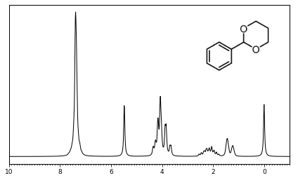
有機系の学生実験で、1H NMR スペクトルの測定を行います。装置の周波数が 60 MHz であるため、シグナルの重なりが頻繁に起こります。そうすると、有機化学の教科書に書いてある通りのスペクトルには見えなくなり、解釈に苦労することになります。例えば、下のスペクトルの 1.4〜2.1 ppm の間のシグナルはどう解釈すればいいのでしょうか。
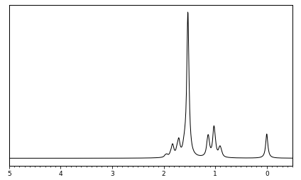
この化合物には、「エチル基」があることがわかっているとしましょう。そうすると、エチルパターン(四重線+三重線)の存在が予想できます。1 ppm 付近に三重線が見えていますから、1.4〜2.1 ppm のところに四重線があるはずです。そこまで考えれば、頭の中でスペクトルを下のように分割して、「四重線と一重線が重なって見えている」という解釈が引き出せます。
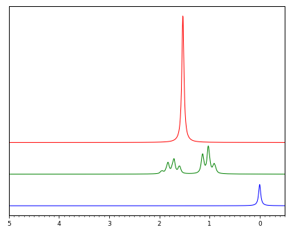
こういう作業は、NMR スペクトルを見慣れてくれば自然にできるようになるのですが、最初は考えるためのヒントが要るかもしれません。上のように、分割したスペクトルと、それを重ねたスペクトルを、それぞれ作図できると役に立ちます。このような図を描くためのツールを見つけました。Python の nmrsim モジュールです。
上の図を描くには、以下のようにコーディングします。まず、エチル基・メチル基・TMS のそれぞれのシグナルを含む Spectrum オブジェクトを作成します。
#  Requirement: nmrsim, numpy, matplotlib

import nmrsim as nmr
import numpy as np
import matplotlib.pyplot as plt
import matplotlib.ticker as ticker

#  Instrument/spectrum settings
freq = 60.0
width = 3
dmax = 5.0
dmin = -0.5
points = 1024

#  Ethyl pattern
delta = np.array([1.76, 1.76, 1.03, 1.03, 1.03])
j = np.array([[0, 0, 7.2, 7.2, 7.2],
              [0, 0, 7.2, 7.2, 7.2],
              [7.2, 7.2, 0, 0, 0],
              [7.2, 7.2, 0, 0, 0],
              [7.2, 7.2, 0, 0, 0]])
ethyl = nmr.SpinSystem(delta * freq, j, w = width)
spec_ethyl = nmr.Spectrum([ethyl], vmin = dmin * freq, vmax = dmax * freq)

#  Methyl and TMS singlets
methyl = nmr.Multiplet(1.53 * freq, 6, [], w = width)
tms = nmr.Multiplet(0, 1, [], w = width)
spec_methyl = nmr.Spectrum([methyl], vmin = dmin * freq, vmax = dmax * freq)
spec_tms = nmr.Spectrum([tms], vmin = dmin * freq, vmax = dmax * freq)
Spectrum オブジェクトの lineshape メソッドを使うと、x 方向・y 方向の数値化データを取得できます。これを matplotlib で描画すればよいのです。
#  Line shapes
spec_x, spec_ethyl_y = spec_ethyl.lineshape(points = points)
_, spec_methyl_y = spec_methyl.lineshape(points = points)
_, spec_tms_y = spec_tms.lineshape(points = points)
ymax = np.max(spec_methyl_y)

#  Draw figures
plt.rcParams.update({'lines.linewidth': 1.0})
plt.rcParams.update({'axes.linewidth': 1.0})
plt.rcParams.update({'font.size': 9})
fig = plt.figure(figsize=(15/2.54, 9/2.54))
ax = fig.add_subplot(111)
ax.plot(spec_x / freq, spec_ethyl_y + spec_methyl_y + spec_tms_y, "k")
ax.set_xlim((dmax, dmin))
ax.xaxis.set_minor_locator(ticker.MultipleLocator(0.1))
ax.yaxis.set_visible(False)
plt.subplots_adjust(top=0.97, left=0.03, right=0.97, bottom=0.08)
plt.savefig("../20250805-01.png", transparent=False, dpi=72)

fig = plt.figure(figsize=(15/2.54, 12/2.54))
ax = fig.add_subplot(111)
ax.plot(spec_x / freq, spec_methyl_y + ymax * 0.5, "r", lw=1)
ax.plot(spec_x / freq, spec_ethyl_y + ymax * 0.25, "g", lw=1)
ax.plot(spec_x / freq, spec_tms_y + ymax * 0, "b", lw=1)
ax.set_xlim((dmax, dmin))
ax.xaxis.set_minor_locator(ticker.MultipleLocator(0.1))
ax.yaxis.set_visible(False)
plt.subplots_adjust(top=0.97, left=0.03, right=0.97, bottom=0.08)
plt.savefig("../20250806-02.png", transparent=False, dpi=72)

plt.show()
上のスペクトルは、エチルパターンと一重線が重なってはいますが、エチルグループのカップリング自体はほぼ一次のスピンカップリング相互作用で解釈できる(ルーフ効果以外)ので、それほど複雑ではありません。一方、次の例は、本当に複雑なスペクトルです。このスペクトルでは、二次のスピンカップリング相互作用と、六員環の立体配座が関与してくるので、考えるべきことが非常に多くなります。ここでは答えは示しません。頑張って解釈しましょう。